Reverse Causality: Spotting False Cause & Effect

Reverse causality, a pervasive issue in fields from econometrics to public health, challenges straightforward cause-and-effect interpretations. The correlation, often misinterpreted, does not inherently prove causation; instead, phenomena like the Simpson's Paradox reveal lurking variables that skew perceived relationships. Understanding this fallacy is vital, especially when analyzing the impact of policies recommended by institutions like the National Institutes of Health (NIH), where interventions might appear successful but actually respond to other underlying factors. Therefore, researchers often use Granger causality which allows them to test whether one time series can forecast another and thus potentially indicate a causal relationship, to avoid the pitfall of reverse causality.

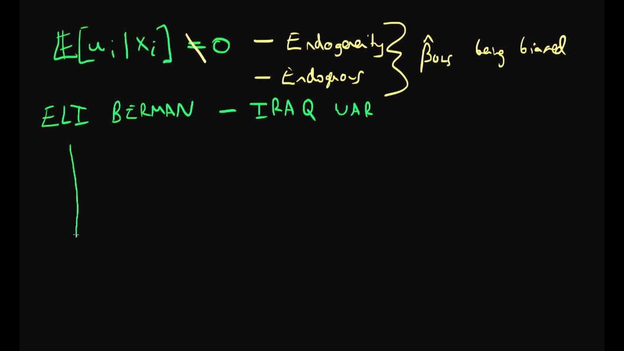
Image taken from the YouTube channel Ben Lambert , from the video titled Reverse Causality - part 1 .

Unveiling the Mysteries of Causation

Understanding causation stands as a cornerstone of progress across nearly all disciplines. From deciphering the intricate mechanisms of disease in medicine to formulating effective economic policies, the ability to discern cause-and-effect relationships is paramount. It is this understanding that allows us to move beyond mere observation and into the realm of prediction and control.

Causation vs. Correlation: A Critical Distinction

At the heart of the matter lies a crucial distinction: causation is not correlation. While correlation indicates a statistical association between two variables, it does not, in itself, prove that one variable causes the other. This is where many analyses falter.

Mistaking correlation for causation can lead to misguided conclusions and ineffective interventions. For example, observing that ice cream sales rise during periods of increased crime does not imply that ice cream consumption causes crime. A third variable, such as warm weather, may be influencing both. This example illustrates the danger of spurious correlations.

Spurious Correlations and the Problem of Confounding

A spurious correlation arises when two variables appear to be related, but their association is, in fact, driven by a third, unobserved variable—a confounding variable. Identifying and controlling for these confounders is one of the major challenges in establishing causal links. Failure to do so can result in drawing wrong conclusions and making poor choices that are not only ineffective but sometimes counter-productive.

Consider a study that finds a positive correlation between coffee consumption and heart disease. Without careful analysis, one might conclude that coffee causes heart disease. However, it's possible that individuals who drink a lot of coffee also tend to smoke more, have poorer diets, or lead more stressful lives. These factors, rather than coffee itself, might be the true drivers of heart disease.

The Challenges of Establishing Causal Links

Establishing genuine causal links is an inherently complex undertaking. The world is a web of interconnected variables, making it difficult to isolate the specific impact of one factor on another. Overcoming this challenge requires a multifaceted approach that includes rigorous experimental design, careful data collection, and sophisticated statistical analysis.

Navigating Causal Inference: Tools and Techniques

To navigate this complex terrain, researchers and analysts rely on a range of causal inference tools. These methodologies are designed to disentangle cause and effect by addressing the problems of confounding and endogeneity. Techniques such as instrumental variable analysis, regression discontinuity designs, and directed acyclic graphs (DAGs) are some examples of these tools.

These tools attempt to approximate the conditions of a controlled experiment, even when a true experiment is not feasible. By leveraging these techniques, we can gain a more accurate understanding of the causal forces at play and make more informed decisions based on reliable causal evidence. The purpose of causal inference tools is to provide a systematic framework for establishing causal relationships.

Core Concepts: Laying the Foundation for Causal Inference

Unveiling the Mysteries of Causation Understanding causation stands as a cornerstone of progress across nearly all disciplines. From deciphering the intricate mechanisms of disease in medicine to formulating effective economic policies, the ability to discern cause-and-effect relationships is paramount. It is this understanding that allows us to model, predict, and, critically, intervene effectively in the complex systems that govern our world. However, before delving into the methodologies used to establish these relationships, we must first solidify our understanding of the fundamental concepts that underpin causal inference.

Defining Causation: Beyond Simple Association

At its heart, causation denotes a relationship between two events where one event (the cause) brings about or produces the other (the effect).

However, this deceptively simple definition belies significant philosophical and practical complexities. We can refine our understanding of causation by considering concepts like necessary and sufficient conditions.

A condition is necessary if the effect cannot occur without it. For example, oxygen is necessary for fire; fire cannot exist without oxygen. A condition is sufficient if its presence guarantees the effect. Lighting a match is usually sufficient for starting a fire, assuming combustible materials are present.

Humean Accounts of Causation

The philosopher David Hume famously challenged our intuitive notions of causation. Hume argued that we only observe constant conjunction – the regular co-occurrence of events – and that our belief in causation is ultimately a matter of psychological habit, not logical necessity. This skeptical perspective underscores the difficulty in definitively proving causal relationships and emphasizes the need for rigorous methods.

The Problem of Endogeneity

A primary challenge in causal inference is endogeneity, a situation where the explanatory variables are correlated with the error term in a regression model. This correlation violates a key assumption of ordinary least squares (OLS) regression, rendering the estimated coefficients biased and inconsistent.

Endogeneity can arise through several mechanisms, each requiring specific remedies.

Omitted Variable Bias and Confounding Variables

Omitted variable bias occurs when a relevant variable that influences both the explanatory and dependent variables is excluded from the model. This omitted variable, often referred to as a confounding variable, creates a spurious relationship between the included variables.

For example, if we observe a correlation between ice cream sales and crime rates, we might erroneously conclude that ice cream consumption causes crime. However, a confounding variable, such as warm weather, likely drives both phenomena.

Simultaneity Bias

Simultaneity bias arises when the explanatory and dependent variables are jointly determined, creating a feedback loop. For example, in a supply and demand model, price affects quantity demanded, and quantity demanded affects price.

This bidirectional relationship makes it difficult to isolate the causal effect of either variable. Addressing simultaneity bias often requires techniques like instrumental variable analysis.

Counterfactuals: Imagining Alternative Realities

Central to modern causal inference is the concept of counterfactuals. A counterfactual is a statement about what would have happened if a different event had occurred. It involves reasoning about alternative scenarios that did not actually take place.

For example, "If I hadn't smoked, I wouldn't have gotten lung cancer" is a counterfactual statement. Counterfactual reasoning allows us to define causal effects as the difference between the observed outcome and the outcome that would have occurred in the absence of the cause.

Counterfactuals and Intervention Evaluation

Counterfactuals are invaluable for evaluating the effects of interventions or treatments. By comparing the observed outcome of a treatment group to the counterfactual outcome – what would have happened to the treatment group had they not received the treatment – we can estimate the causal effect of the intervention.

Of course, we cannot directly observe counterfactuals, as they represent hypothetical scenarios. Therefore, causal inference methods aim to approximate these counterfactual outcomes using various statistical techniques, paving the way for data-driven, rigorous policy evaluation.

Methodologies: The Toolkit for Causal Exploration

Having laid the foundational concepts, we now turn to the practical methodologies that empower researchers to explore causal relationships. These tools, while varied in their approach, share a common goal: to isolate the true effect of one variable on another, disentangling causation from mere correlation.

Instrumental Variable (IV) Analysis

Instrumental Variable (IV) analysis is a powerful technique employed to address the pervasive problem of endogeneity. Endogeneity arises when the independent variable of interest is correlated with the error term in a regression model, leading to biased estimates.

IV analysis offers a way out by leveraging an instrument – a variable that is correlated with the endogenous independent variable, but is independent of the error term.

Solving Endogeneity with IVs

The core idea is that the instrument influences the independent variable, which, in turn, affects the dependent variable. By using the instrument to isolate the variation in the independent variable that is not correlated with the error term, we can obtain a more accurate estimate of the causal effect.

Criteria for Valid Instruments

For an instrument to be valid, it must satisfy two key criteria:

• Relevance: The instrument must be strongly correlated with the endogenous independent variable. This can be tested statistically.

• Exogeneity: The instrument must be independent of the error term in the regression model. This is a more challenging assumption to verify, as it requires that the instrument only affects the dependent variable through its effect on the independent variable.

Natural Experiments

Natural experiments offer a unique opportunity to study causal relationships in settings where controlled experiments are infeasible or unethical. These experiments exploit naturally occurring events or policy changes that resemble randomized interventions.

Approximating Controlled Experiments

By carefully analyzing the effects of these "natural treatments," researchers can gain insights into causal effects. The key is to identify a control group that is similar to the treatment group, but was not exposed to the intervention.

Examples of Natural Experiments

A classic example is the study of the effect of education on earnings, where researchers have used changes in compulsory schooling laws as a natural experiment. Other examples include policy changes, environmental events, or even the random assignment of judges to cases.

Granger Causality Test

The Granger causality test is a statistical method used to determine if one time series can predict another. If a time series X "Granger-causes" another time series Y, it means that past values of X contain information that helps predict Y above and beyond the information contained in past values of Y alone.

Granger Causality for Time Series Data

The test involves regressing Y on its own past values and on the past values of X. If the coefficients on the past values of X are statistically significant, then X is said to Granger-cause Y.

Limitations

It is crucial to remember that Granger causality does not necessarily imply true causation. It only indicates predictive precedence. There may be a third variable that is driving both X and Y, or the relationship may be spurious. The test is best used as an exploratory tool, rather than as definitive proof of causation.

Propensity Score Matching

Propensity Score Matching (PSM) is a statistical technique used to estimate the effect of a treatment or intervention by accounting for the covariates that predict receiving the treatment.

Estimating Treatment Effects

The propensity score is the probability of receiving the treatment given a set of observed characteristics.

PSM involves matching treated and untreated individuals who have similar propensity scores, effectively creating a control group that is comparable to the treatment group. The treatment effect is then estimated by comparing the outcomes of the matched individuals.

Difference-in-Differences (DID)

Difference-in-Differences (DID) is a quasi-experimental technique used to estimate the effect of a treatment or intervention by comparing the changes in outcomes over time between a treatment group and a control group.

Comparing Treatment and Control Groups

The key assumption of DID is that, in the absence of the treatment, the treatment and control groups would have followed parallel trends. The treatment effect is estimated by taking the difference in the changes in outcomes between the two groups.

Regression Discontinuity Design (RDD)

Regression Discontinuity Design (RDD) is a quasi-experimental method used to estimate the causal effect of a treatment or intervention when eligibility for the treatment is determined by a cutoff score on a continuous variable.

Measuring Treatment Effects

Individuals just above the cutoff receive the treatment, while those just below do not. By comparing the outcomes of individuals on either side of the cutoff, researchers can estimate the local average treatment effect. RDD relies on the assumption that individuals close to the cutoff are similar in all other respects, so any difference in outcomes can be attributed to the treatment.

Directed Acyclic Graphs (DAGs)

Directed Acyclic Graphs (DAGs) are graphical models that represent causal relationships between variables. They consist of nodes, representing variables, and directed edges, representing causal effects.

Visualizing Causal Structures

The absence of an edge between two nodes implies that there is no direct causal effect between them. DAGs are acyclic, meaning that there are no feedback loops.

DAGs in Designing Causal Studies

DAGs are a valuable tool for designing causal studies, as they can help researchers identify potential confounders and mediators, and to select appropriate statistical methods for estimating causal effects. They provide a visual framework for understanding the complex relationships between variables and for making informed decisions about causal inference.

Pioneers of Causality: Honoring Influential Thinkers

Having laid the foundational concepts, we now turn to the practical methodologies that empower researchers to explore causal relationships. But behind every methodology lies a foundation of theoretical breakthroughs and paradigm-shifting insights. This section pays homage to some of the towering figures who have shaped our understanding of causation, leaving an indelible mark on the field.

David Hume: The Skeptical Empiricist

David Hume, the 18th-century Scottish philosopher, stands as a pivotal figure in the history of causal thought. Hume's skeptical empiricism challenged the prevailing notions of causation. He argued that we can never truly perceive a necessary connection between cause and effect.

Instead, Hume posited that our understanding of causation arises from the constant conjunction of events. We observe event A consistently followed by event B, and from this repeated experience, we infer a causal relationship.

However, Hume cautioned that this inference is ultimately based on habit and custom, not on any inherent causal power. His rigorous questioning of causal certainty laid the groundwork for future investigations into the nature of causal inference.

John Stuart Mill: Systematizing Causal Inquiry

A century later, John Stuart Mill sought to systematize the process of identifying causes. His "Mill's Methods," outlined in his A System of Logic, provided a structured approach to causal discovery.

Mill identified five methods, each designed to isolate the causal factor in a given phenomenon:

• Method of Agreement: Identifying a common factor present in all instances where the effect occurs.
• Method of Difference: Observing the absence of the effect when a specific factor is absent, while all other factors remain constant.
• Joint Method of Agreement and Difference: Combining the strengths of the first two methods.
• Method of Residues: Subtracting known causal effects to isolate the cause of the remaining effect.
• Method of Concomitant Variations: Observing how changes in one factor correlate with changes in another.

While Mill's Methods offer a valuable framework, they are not without limitations. They assume that the possible causes are already known and that the causal relationships are deterministic. Nevertheless, they remain a cornerstone of causal reasoning, particularly in the early stages of investigation.

Judea Pearl: Revolutionizing Causal Inference

Judea Pearl, a towering figure in modern causal inference, has revolutionized the field with his development of graphical models and the do-calculus. Pearl introduced Directed Acyclic Graphs (DAGs) as a powerful tool for representing causal relationships visually.

DAGs allow researchers to encode their assumptions about the causal structure of a system, explicitly representing the relationships between variables.

Furthermore, Pearl developed the do-calculus, a set of rules for manipulating causal models and answering counterfactual questions. The do-calculus provides a formal framework for reasoning about interventions. These interventions allow us to predict the effects of manipulating variables within a causal system.

Pearl's work has had a profound impact on numerous fields, providing a rigorous and intuitive framework for causal inference.

Imbens and Angrist: The Credibility Revolution

Guido Imbens and Joshua Angrist are celebrated for their pioneering work in instrumental variables and quasi-experimental methods. Their contributions have ushered in what is often referred to as the "credibility revolution" in econometrics.

Imbens and Angrist emphasized the importance of clearly identifying causal effects using credible research designs.

Their work on local average treatment effects (LATE) provided a framework for understanding the causal effects of interventions in specific subpopulations. In 2021, Imbens and Angrist were awarded the Nobel Prize in Economics for their methodological contributions to the analysis of causal relationships. Their work has provided researchers with a toolkit for drawing more robust and reliable causal inferences from observational data.

These are just a few of the many brilliant minds who have contributed to our understanding of causation. Their insights continue to shape the field, inspiring new generations of researchers to unravel the mysteries of cause and effect.

Causal Inference in Action: Real-World Applications

Having explored the theoretical foundations and celebrated the pioneers of causal inference, it is crucial to demonstrate the practical applications that highlight its significance. Causal inference transcends theoretical exercises; it is a powerful tool that provides insights in various fields, allowing us to understand and potentially alter the course of events in economics, epidemiology, medicine, public health, and the social sciences.

Causal Inference in Economics

Economics, particularly the sub-discipline of econometrics, heavily relies on causal inference to understand economic phenomena. The challenge lies in distinguishing correlation from causation in inherently observational data.

For example, one might observe that higher education levels are associated with higher income. Is this a causal relationship? Does more education cause higher income, or are other factors at play, such as innate ability or family background?

Econometricians employ techniques such as instrumental variable (IV) analysis and regression discontinuity design (RDD) to address endogeneity and uncover causal relationships. These methods allow for the evaluation of policy interventions, such as the impact of minimum wage laws on employment, or the effect of tax incentives on investment.

The rigorous application of causal inference methods is what allows for evidence-based policy recommendations.

Epidemiology: Unraveling the Causes of Disease

Epidemiology aims to identify the causes and risk factors associated with diseases. Establishing causal relationships is vital for designing effective public health interventions and preventive strategies.

It's easy to note correlations—observing that people who drink coffee are less likely to develop a particular disease. But is coffee causally protective, or is this association due to other lifestyle factors correlated with coffee consumption?

Epidemiologists utilize various causal inference methods, including cohort studies, case-control studies, and Mendelian randomization, to disentangle these complex relationships. Mendelian randomization, in particular, uses genetic variants as instrumental variables to assess the causal effects of modifiable risk factors on disease outcomes.

By identifying causal factors, epidemiologists can effectively advise public health initiatives and mitigate the impact of widespread illnesses.

Evaluating Treatment Effectiveness in Medicine and Public Health

In medicine and public health, causal inference is indispensable for evaluating the effectiveness of treatments, interventions, and healthcare policies. Clinical trials, with their random assignment of participants to treatment and control groups, are a cornerstone of causal inference in this field.

However, challenges arise when randomized controlled trials are not feasible or ethical. For instance, assessing the long-term effects of a public health campaign on smoking cessation requires careful consideration of potential confounding factors.

Methods like propensity score matching and difference-in-differences are employed to address these challenges, allowing researchers to make causal claims. By rigorously evaluating the impacts of medical interventions, researchers can improve healthcare outcomes and inform evidence-based medical practice.

Social Sciences: Understanding Social Phenomena

In the social sciences, causal inference is vital for understanding complex social phenomena, from the effects of social programs on poverty reduction to the impact of media exposure on political attitudes. Social scientists often grapple with observational data and a multitude of confounding factors.

Consider the effect of a community policing initiative on crime rates. A simple comparison of crime rates before and after the intervention may be misleading due to external factors.

Researchers use causal inference techniques like regression analysis with control variables, instrumental variables, and natural experiments to estimate the causal effects of social interventions. Directed acyclic graphs (DAGs) also help in visualizing and understanding the potential causal relationships among variables.

These methods contribute to the development of effective social policies and improve the understanding of social dynamics. By identifying the causes of social problems, social scientists play a crucial role in informing policy decisions and improving societal well-being.

Video: Reverse Causality: Spotting False Cause & Effect

Play Video

So, next time you see a headline screaming about some connection between two things, take a beat. Don't automatically assume A causes B. Maybe, just maybe, B is actually causing A. Keep an eye out for that sneaky reverse causality – it could save you from making some pretty big assumptions!