Median vs Mean: Differences & When to Use Which

In statistical analysis, the mean serves as the arithmetic average, calculated by summing all values and dividing by the number of values, whereas the median identifies the central data point, effectively splitting the dataset into two equal halves, an important concept when examining measures of central tendency. Data analysts frequently utilize software tools like SPSS to compute both these measures in order to derive actionable insights. The application of either median or mean is largely dependent on the data distribution, and this decision-making process is particularly relevant when dealing with datasets exhibiting outliers, which can disproportionately skew the mean, a phenomenon often discussed in academic circles and publications from organizations like the American Statistical Association.

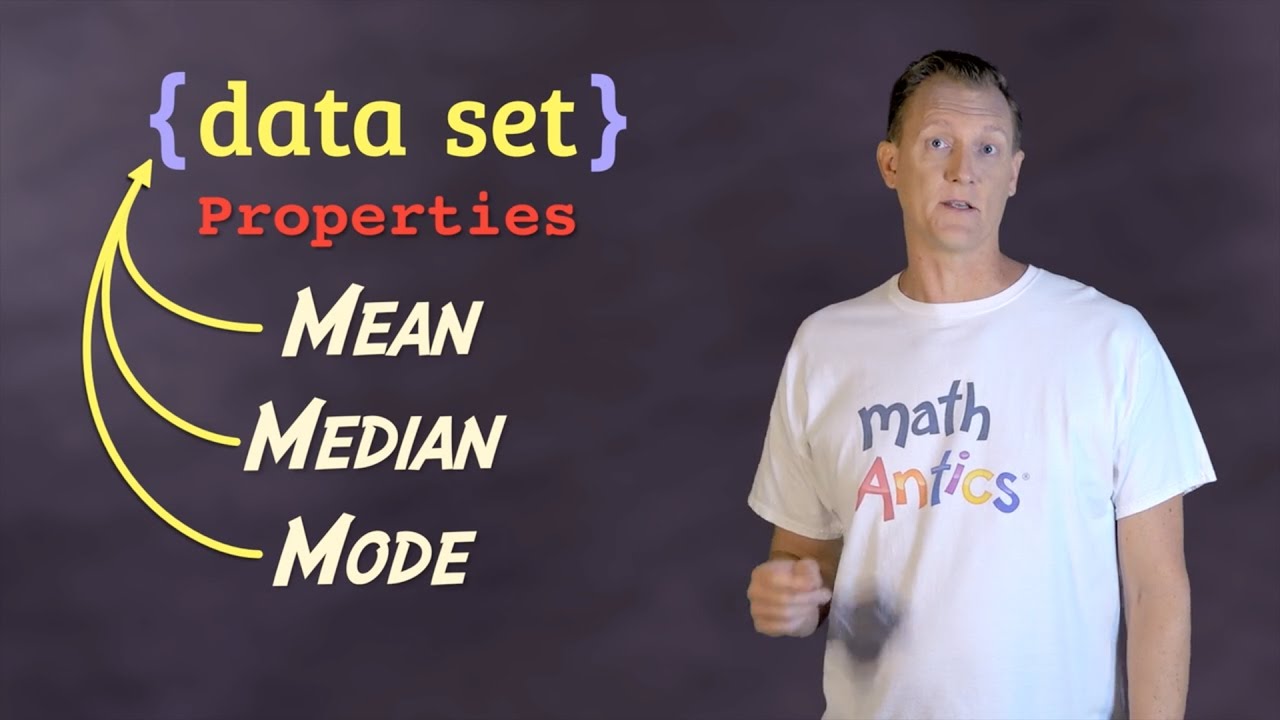
Image taken from the YouTube channel Whats Up Dude , from the video titled The Average Or Mean VS The Median - Difference Between The Mean And The Median .

Demystifying Averages: Unveiling the Power of Mean and Median

Averages are ubiquitous. We encounter them daily, from average temperatures and travel times to average salaries and customer ratings. But what is an average, and why should we care? At its core, an average is a measure of central tendency—a single value that attempts to describe a set of data by identifying its "typical" value.

Central Tendency: Finding the Heart of the Data

The purpose of central tendency is to provide a concise summary of a dataset, enabling us to quickly grasp its general characteristics. Without such measures, we would be forced to sift through raw, often overwhelming, data points, making meaningful interpretations nearly impossible.

Imagine trying to understand the performance of a class on an exam without calculating the average score. Central tendency provides a valuable tool for data reduction and informed decision-making.

Why Averages Matter: Navigating the Data Landscape

Understanding averages, specifically the mean and the median, is crucial for anyone who interacts with data. In an increasingly data-driven world, the ability to interpret and analyze information is paramount.

These statistical measures provide a foundation for making sound judgments. Averages can reveal trends, identify outliers, and facilitate comparisons across different datasets. They inform business strategies, policy decisions, and even personal choices.

Mean and Median: Two Sides of the Same Coin

While both the mean and the median fall under the umbrella of "averages," they represent distinct methods of calculating central tendency. The mean, often referred to as the arithmetic average, is calculated by summing all values in a dataset and dividing by the number of values.

The median, on the other hand, represents the middle value in a dataset that has been ordered from least to greatest. These two measures can provide different insights into the data, particularly when dealing with skewed distributions or outliers.

The Practical Power of Averages: Applications Across Domains

The practical applications of understanding and calculating averages are vast and varied. In finance, averages are used to track market trends and assess investment performance. In healthcare, they help monitor patient vital signs and evaluate the effectiveness of treatments.

In marketing, averages can gauge customer satisfaction and optimize advertising campaigns. The ability to calculate and interpret averages is a valuable skill in nearly every profession, and in daily life.

Whether you're a student, a business professional, or simply a curious individual, grasping the nuances of averages will empower you to make more informed decisions and navigate the complexities of the data-rich world around us.

The Arithmetic Mean: Calculation and Applications

Having introduced the broad concept of averages, we now delve into the arithmetic mean, often simply referred to as the "average." Understanding its calculation and appropriate usage is paramount for sound data interpretation.

Defining the Arithmetic Mean

The arithmetic mean is the sum of a collection of numbers divided by the count of numbers in the collection.

In mathematical terms, if we have a dataset consisting of 'n' values: x₁, x₂, x₃, ..., x_n, then the arithmetic mean (represented as μ for a population and x̄ for a sample) is calculated as:

μ = (x₁ + x₂ + x₃ + ... + x_n) / n

This provides a single value that represents the "center" of the data in a specific way.

Calculating the Mean: A Practical Demonstration

To illustrate, let's consider a simple example. Suppose we have the following set of test scores: 75, 80, 85, 90, and 95.

To calculate the arithmetic mean, we sum these scores: 75 + 80 + 85 + 90 + 95 = 425.

Then, we divide by the number of scores, which is 5: 425 / 5 = 85.

Therefore, the arithmetic mean of these test scores is 85.

When to Employ the Arithmetic Mean

The arithmetic mean is a suitable measure of central tendency when dealing with data that is relatively evenly distributed and lacks significant outliers.

For instance, it's commonly used to calculate:

• Average test scores for a class.
• Average height of individuals in a population.
• Average daily temperature over a period.

In these scenarios, the mean provides a reasonable representation of the "typical" value.

The Achilles' Heel: Sensitivity to Extreme Values

It is crucial to acknowledge that the arithmetic mean is highly sensitive to extreme values, also known as outliers.

A single very large or very small value can significantly skew the mean, making it a less representative measure of central tendency.

Consider the following example: Salaries of employees in a small company are $40,000, $45,000, $50,000, $60,000, and $500,000 (the CEO's salary).

The arithmetic mean is $139,000. This value is significantly higher than most of the employees' salaries, making it a misleading representation of the typical salary.

In such cases, alternative measures like the median provide a more robust and informative representation.

The sensitivity of the mean to outliers underscores the importance of understanding the distribution of the data before choosing which measure of central tendency to use. Always consider if extreme values could disproportionately influence the average and potentially misrepresent the typical value.

The Median: Finding the Middle Ground

Having explored the arithmetic mean, it's time to turn our attention to another crucial measure of central tendency: the median. The median offers a different perspective on the "average," particularly valuable when dealing with datasets that might be skewed or contain outliers. Understanding its calculation and application is essential for a comprehensive understanding of data analysis.

Understanding the Median: The Middle Value

The median represents the middle value in a dataset that has been ordered from least to greatest. It's the point that divides the distribution exactly in half, with 50% of the data points falling below and 50% falling above.

Unlike the mean, which is calculated by summing all values and dividing by the number of values, the median is determined by position. This positional characteristic makes the median particularly useful in certain situations, as we'll explore.

Calculating the Median: Odd and Even Datasets

Calculating the median requires slightly different approaches depending on whether the dataset contains an odd or even number of values.

Odd Number of Values

When the dataset contains an odd number of values, finding the median is straightforward. Simply arrange the data in ascending order, and the median is the value that sits exactly in the middle.

For example, consider the dataset: [2, 5, 8, 12, 15]. The median is 8, as it is the central value with two values below it and two values above it.

Even Number of Values

When the dataset contains an even number of values, the median is calculated as the average of the two middle values.

First, arrange the data in ascending order. Then, identify the two values that sit closest to the middle. The median is the sum of these two values divided by two.

For example, consider the dataset: [2, 5, 8, 12]. The two middle values are 5 and 8. The median is (5 + 8) / 2 = 6.5.

When the Median Shines: Robustness Against Outliers

The median's key advantage lies in its robustness against outliers. Outliers are extreme values that deviate significantly from the rest of the data. The mean is highly sensitive to outliers, as their values directly influence the sum used in the calculation.

The median, however, is largely unaffected by outliers. Because it is based on position rather than value, extreme values do not disproportionately impact the median. They only affect the values at the extreme ends of the ordered dataset, leaving the middle value relatively stable.

Consider, for instance, a dataset representing income levels in a population: [20000, 30000, 40000, 50000, 1000000].

The mean income would be heavily inflated by the single high earner, giving a misleading impression of the typical income level. The median, however, would provide a more accurate representation of the central tendency, effectively ignoring the outlier.

Therefore, the median is often the preferred measure when dealing with data that is likely to contain outliers or is heavily skewed, providing a more representative view of the "typical" value. It is vital in scenarios where an accurate representation of the central data is crucial.

Beyond the Basics: Exploring Other Types of Averages

While the arithmetic mean and median often serve as the primary tools for summarizing data, they represent only a subset of the averaging techniques available. A deeper understanding of data analysis requires familiarity with alternative methods, each designed to address specific analytical challenges. Let's explore three such alternatives: the weighted average, the geometric mean, and the harmonic mean, each offering unique insights when applied appropriately.

Weighted Average: Accounting for Varying Importance

The weighted average, also known as the weighted mean, is a crucial tool when certain data points carry more significance than others.

Unlike the arithmetic mean, which treats all values equally, the weighted average assigns different weights to each value, reflecting its relative importance.

This is particularly useful in scenarios such as calculating a student's grade point average (GPA), where different courses have different credit hours.

Calculating the Weighted Average

The formula for calculating the weighted average is:

Weighted Average = (∑(Weight

**Value)) / ∑(Weight)

Where:

• ∑ represents the summation.
• Weight is the assigned weight to each value.
• Value is the data point itself.

Example: Calculating a Weighted Grade

Consider a student taking three courses: Math (4 credits), Science (3 credits), and English (3 credits). The student earns an A (4.0) in Math, a B (3.0) in Science, and a C (2.0) in English.

The weighted GPA would be calculated as follows:

Weighted GPA = ((4 4.0) + (3 3.0) + (3** 2.0)) / (4 + 3 + 3) = 3.1

This result provides a more accurate representation of the student's overall performance by considering the different credit weights of each course.

Geometric Mean: Measuring Growth Over Time

The geometric mean is a specialized average primarily used to calculate the average growth rate over a period of time. It's particularly useful when dealing with percentages or rates of change.

Unlike the arithmetic mean, which can be misleading in such scenarios, the geometric mean accurately reflects the compounding effect of growth.

When to Use the Geometric Mean

The geometric mean shines when analyzing financial returns, population growth, or any situation involving multiplicative changes.

It ensures that the average growth rate accurately reflects the overall change over the entire period.

Calculation Example

Imagine an investment that grows by 10% in the first year, 20% in the second year, and 30% in the third year.

To calculate the average annual growth rate using the geometric mean:

1. Add 1 to each growth rate: 1.10, 1.20, 1.30
2. Multiply these values together: 1.10 1.20 1.30 = 1.716
3. Take the nth root, where n is the number of periods (in this case, 3): ∛1.716 ≈ 1.197
4. Subtract 1 to get the average growth rate: 1.197 - 1 = 0.197 or 19.7%

The average annual growth rate is approximately 19.7%, a more accurate representation than the arithmetic mean would provide.

Harmonic Mean: Averaging Rates and Ratios

The harmonic mean is specifically designed for averaging rates or ratios. It is particularly useful when dealing with situations where the denominator remains constant.

Use Cases for the Harmonic Mean

A classic example is calculating the average speed of a vehicle traveling the same distance at different speeds. The harmonic mean ensures that the average accurately reflects the total distance traveled and the total time taken.

Calculation Example

Suppose a car travels 120 miles. It travels the first 60 miles at 30 mph and the second 60 miles at 60 mph. The harmonic mean is used to find the average speed.

The formula is:

Harmonic Mean = n / (∑(1 / Value))

Where:

• n is the number of values.
• Value represents each individual rate or ratio.

In this case:

Harmonic Mean = 2 / ((1/30) + (1/60)) = 2 / (0.0333 + 0.0167) = 2 / 0.05 = 40 mph

Therefore, the average speed for the entire trip is 40 mph. This accurately accounts for the time spent traveling at each speed, providing a more realistic average than a simple arithmetic mean.

Mean vs. Median: Choosing the Right Measure

While the arithmetic mean and median often serve as the primary tools for summarizing data, they represent only a subset of the averaging techniques available. A deeper understanding of data analysis requires familiarity with alternative methods, each designed to address specific analytical challenges. To effectively interpret data, it is essential to discern when to use the mean and when the median provides a more accurate representation. Several key factors come into play in making this determination, most notably the presence of outliers, the skewness of the data distribution, and the overall shape of the dataset.

The Impact of Outliers

Outliers, those extreme values that deviate significantly from the bulk of the data, can exert a disproportionate influence on the mean. Because the mean considers every value in the dataset, these extreme points can skew the average upwards or downwards, making it less representative of the "typical" value.

Consider a dataset of housing prices in a particular neighborhood. If a few multi-million dollar mansions are included, they can substantially inflate the mean house price, giving a misleading impression of affordability.

In contrast, the median is far more robust in the face of outliers. As the middle value in an ordered dataset, the median is unaffected by the magnitude of extreme values. It only cares about the number of values above and below it.

In the housing price example, the median house price would likely provide a more accurate reflection of what a typical home costs in that neighborhood, as it is not unduly influenced by the presence of a few very expensive properties.

Skewness and Its Effect

Skewness refers to the asymmetry of a data distribution. A symmetrical distribution, like the normal distribution, has a balanced shape with the mean and median coinciding at the center. However, many real-world datasets are not symmetrical; they exhibit skewness, which affects the relationship between the mean and median.

In a positively skewed distribution, also known as a right-skewed distribution, the tail extends towards higher values. This is common in datasets like income, where a small number of individuals earn significantly more than the majority.

In this scenario, the mean is typically greater than the median. The high values in the tail pull the mean upwards, while the median remains closer to the center of the data cluster.

Conversely, in a negatively skewed distribution, also known as a left-skewed distribution, the tail extends towards lower values.

An example could be the age of retirement in a population where many people retire early. Here, the mean is usually less than the median, as the low values in the tail pull the mean downwards.

Understanding the direction and magnitude of skewness is crucial for selecting the appropriate measure of central tendency.

Understanding Data Distribution

The overall distribution of the data plays a critical role in determining whether the mean or median is the more appropriate measure. A normal distribution is characterized by its bell shape, with the mean, median, and mode all being equal and located at the center. In this ideal scenario, both the mean and median provide an equally accurate representation of the "typical" value.

However, many datasets do not conform to a normal distribution.

In situations where the distribution is asymmetrical, such as those exhibiting skewness or containing outliers, the median often provides a more stable and reliable measure of central tendency.

A frequency distribution is a visual representation of how often each value (or range of values) occurs in a dataset. Histograms and frequency tables are common ways to depict frequency distributions. Examining the frequency distribution can quickly reveal the presence of skewness or outliers.

A long tail on one side indicates skewness, while isolated bars far from the main cluster of data points suggest the presence of outliers. By visualizing the distribution, you can make a more informed decision about whether the mean or median is the more appropriate summary statistic.

Real-World Applications: Mean and Median in Action

While the arithmetic mean and median often serve as the primary tools for summarizing data, their indiscriminate application can lead to misleading conclusions. A deeper understanding of data analysis requires a nuanced approach, recognizing when each measure provides the most accurate and representative insight. To illustrate the critical importance of this distinction, let's examine several real-world scenarios where the choice between mean and median significantly impacts the interpretation of data.

Income Distribution: The Skew of Wealth

One of the most common and compelling examples is income distribution. When analyzing the economic well-being of a population, the median income is almost always the preferred metric. This is because income distributions are often highly skewed, with a long tail of high earners pulling the mean income upward.

Consider a scenario where a small percentage of the population earns extremely high incomes. These outliers significantly inflate the mean, creating a distorted picture of the "typical" income. The median, representing the income level at which half the population earns more and half earns less, provides a more accurate reflection of the economic experience of the majority.

The median income effectively mitigates the influence of extreme values, offering a more balanced representation of the financial reality for most individuals. Using the mean income in this context can create a false impression of widespread prosperity, masking the true extent of income inequality.

Housing Prices: Gauging the Market

Similar to income distribution, housing prices often exhibit skewness, particularly in markets with a concentration of luxury properties. The mean house price can be heavily influenced by a few exceptionally expensive homes, leading to an overestimation of typical housing costs.

Imagine a neighborhood where a handful of multi-million dollar mansions exist alongside more modest, family-sized homes. The mean house price will be significantly higher than what most people in that area actually pay for their homes.

Therefore, the median house price provides a more accurate representation of the "typical" home value, reflecting the prices of homes that are more representative of the market as a whole. Potential homebuyers and real estate analysts often rely on the median to understand true market trends.

Test Scores: Understanding Performance

The choice between mean and median in analyzing test scores depends heavily on the distribution of the scores. In a perfectly symmetrical distribution, where scores are evenly distributed around the average, the mean and median will be nearly identical and can be used interchangeably.

However, if the distribution is skewed—for example, with a cluster of high scores and a tail of lower scores—the mean will be pulled towards the higher end, potentially misrepresenting the performance of the majority of students. If most students scored poorly, a few high scores could make it appear like they are doing well.

In such cases, the median score might offer a more accurate reflection of the "typical" performance level. If there are a few extreme outliers or skewed data, the median can also be used to indicate the central tendency.

Reaction Times in Experiments: Taming the Outliers

In scientific experiments, particularly those measuring reaction times, outliers are a common occurrence. A participant might be momentarily distracted, resulting in an unusually long reaction time. These extreme values can significantly inflate the mean reaction time.

As the median is more resistant to the influence of outliers, researchers often prefer it as a measure of central tendency.

It provides a more stable and representative estimate of typical reaction times, less susceptible to distortion by occasional lapses in attention or equipment glitches. This ensures a more reliable and accurate interpretation of the experimental results.

Website Loading Times: A Better User Experience Metric

For website owners, website loading time is a critical factor in user experience. While the mean loading time might seem like a useful metric, it can be misleading due to occasional slow loading times caused by server issues or network congestion.

A few instances of extremely slow loading can dramatically increase the mean, even if most users experience relatively fast loading times. Consequently, the median loading time gives a more accurate picture of the typical user experience.

The median better reflects the loading times encountered by the majority of visitors, providing a more reliable indicator of website performance and potential usability issues. It will also help prioritize website maintenance and identify possible downtimes.

Salary Negotiations: Know Your Worth

In salary negotiations, both the mean and median salary data can be valuable tools, but they should be used strategically and with a clear understanding of their limitations.

Understanding the mean salary for a position in a specific industry and location can provide a general benchmark. However, it's crucial to recognize that this number may be skewed by exceptionally high earners.

The median salary offers a more realistic assessment of the "typical" salary for that role, helping you gauge a fair market rate based on experience and qualifications. Highlighting your skills can move your pay closer to the median.

Tools for Calculating Averages: Making it Easier

While understanding the concepts of mean and median is crucial, the actual calculation, especially with large datasets, can be cumbersome. Fortunately, a variety of tools are available to streamline this process, ranging from simple spreadsheet software to sophisticated statistical packages. These tools not only automate calculations but also offer features for data visualization and in-depth analysis. Selecting the right tool depends on the complexity of the data and the specific analytical goals.

Spreadsheet Software: Accessible and User-Friendly

Spreadsheet programs like Microsoft Excel and Google Sheets are widely accessible and provide a user-friendly environment for basic statistical calculations. Their intuitive interface makes them ideal for individuals with limited statistical expertise.

Basic Formulas for Mean and Median

Excel and Google Sheets allow users to calculate the mean and median using simple formulas. The formula =AVERAGE(range) calculates the arithmetic mean of the values within the specified range. For example, =AVERAGE(A1:A100) computes the average of the values in cells A1 through A100.

To find the median, the formula =MEDIAN(range) is used. Similarly, =MEDIAN(A1:A100) returns the median value of the data in cells A1 to A100. These basic formulas provide a quick and easy way to determine these measures of central tendency.

Built-in Functions for Efficiency

Beyond basic formulas, spreadsheet software offers built-in functions that simplify the process of calculating averages. These functions handle the underlying logic, making it easy for users to obtain the desired results without manually implementing complex algorithms. This ease of use makes spreadsheet software an excellent starting point for data analysis.

Statistical Software Packages: Power and Precision

For more complex statistical analyses, dedicated statistical software packages like R, Python (with libraries like NumPy and Pandas), SPSS, SAS, and Stata offer a comprehensive suite of tools. These packages provide advanced functionalities for data manipulation, statistical modeling, and visualization.

Handling Complex Statistical Analyses

Statistical software packages are designed to handle large and complex datasets. They offer a wide range of statistical methods, including hypothesis testing, regression analysis, and time series analysis. These tools allow researchers and analysts to perform sophisticated analyses that go beyond the capabilities of spreadsheet software.

Visual Representations of Data Distributions

One of the key strengths of statistical software packages is their ability to create visually appealing and informative representations of data distributions. Histograms, box plots, and scatter plots can be easily generated to gain insights into the shape, center, and spread of the data. Visualizations aid in understanding the characteristics of the data and identifying patterns or anomalies.

Descriptive and Robust Statistics

Statistical software packages provide tools for calculating both descriptive and robust statistics. Descriptive statistics, such as the mean, median, standard deviation, and variance, summarize the key features of the data.

Robust statistics are less sensitive to outliers and provide more reliable measures of central tendency and spread when the data contains extreme values. These packages empower users to choose the most appropriate statistical methods for their specific data and analytical objectives.

Descriptive Statistics: Summarizing Your Data

Tools for Calculating Averages: Making it Easier

While understanding the concepts of mean and median is crucial, the actual calculation, especially with large datasets, can be cumbersome. Fortunately, a variety of tools are available to streamline this process, ranging from simple spreadsheet software to sophisticated statistical packages. These tools output important descriptive statistics, including mean and median.

Descriptive statistics are essential for summarizing and understanding the key characteristics of a dataset. They provide a concise overview, allowing us to grasp the central tendencies, dispersion, and shape of the data distribution. By employing descriptive statistics, we can transform raw data into meaningful insights, facilitating informed decision-making and further analysis.

Utilizing Descriptive Statistics for Data Summarization

Descriptive statistics allow us to condense large amounts of data into manageable and interpretable summaries. This involves identifying key features, such as the average value, the spread of data points, and the presence of any skewness or outliers.

Measures of central tendency, such as the mean and median, provide information about the typical or central value in a dataset. The mean, as discussed previously, is sensitive to extreme values, while the median offers a more robust measure in the presence of outliers.

Understanding the distribution of data is crucial. This can be achieved through measures of spread, such as the standard deviation and interquartile range (IQR).

The standard deviation quantifies the average distance of data points from the mean, providing a measure of overall variability.

The IQR, on the other hand, represents the range within which the middle 50% of the data falls, offering a robust measure of spread that is less affected by outliers.

The Role of Robust Statistics

Traditional descriptive statistics, such as the mean and standard deviation, can be heavily influenced by outliers, potentially leading to misleading conclusions. Robust statistics offer alternative methods that are less sensitive to extreme values, providing a more accurate representation of the underlying data.

For example, instead of the mean, the trimmed mean can be used, which involves removing a certain percentage of the highest and lowest values before calculating the average. This reduces the impact of outliers on the final result.

Similarly, the median absolute deviation (MAD) is a robust measure of spread that is less affected by extreme values compared to the standard deviation.

Measures of Spread Combined with Central Tendency

To gain a comprehensive understanding of a dataset, it is essential to consider measures of spread in conjunction with measures of central tendency. Knowing the mean or median alone provides limited information.

For example, a dataset with a high standard deviation indicates that the data points are widely dispersed around the mean. This suggests greater variability and uncertainty compared to a dataset with a low standard deviation.

The IQR can be used to identify potential outliers. Data points that fall significantly outside the IQR may warrant further investigation.

By combining measures of central tendency and spread, we can create a more complete and nuanced picture of the data, enabling us to draw more accurate conclusions and make better informed decisions. Visualizations like box plots can effectively display both central tendency and spread, providing a quick and informative overview of the data distribution.

Video: Median vs Mean: Differences & When to Use Which

Play Video

So, next time you're staring down a dataset and wondering which average to use, remember the key differences between the median vs mean. Consider what you're trying to highlight and whether outliers might be skewing the picture. With a little thought, you'll be able to choose the right tool for the job and confidently present your data.