Mastering Maclaurin Series of cos(x): The Ultimate Guide

The Maclaurin series, a specific type of Taylor series, provides a powerful method for approximating functions. Maclaurin series of cos(x), a prominent application, allows us to represent the cosine function as an infinite polynomial. Calculus serves as the foundational framework for understanding these series, enabling the derivation and manipulation of trigonometric functions. Wolfram Alpha, a computational knowledge engine, offers tools to readily calculate and visualize the Maclaurin series approximations, making complex mathematics more accessible.

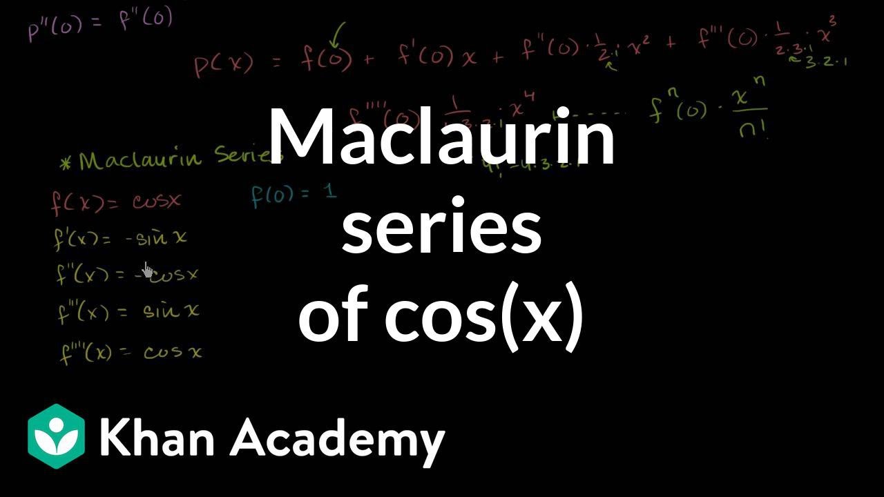
Image taken from the YouTube channel Khan Academy , from the video titled Maclaurin series of cos(x) | Series | AP Calculus BC | Khan Academy .

The Maclaurin series stands as a cornerstone of calculus, a powerful tool that allows us to represent a wide range of functions as infinite sums of terms. This representation, seemingly abstract, has profound implications for approximating function values and simplifying complex mathematical problems.

In essence, the Maclaurin series provides a polynomial approximation of a function around the point x = 0. This is particularly useful when dealing with functions that are difficult to compute directly or when a simplified representation is needed for analytical purposes.

The Significance of Series Representations

Functions can be represented in a lot of ways, but series representations are especially useful. They change a function into an infinite sum of terms, usually involving powers of x. This approach is especially useful for:

• Approximation: Series allow accurate approximations of function values, especially when direct computation is challenging or impossible.

• Computation: Series simplify calculations, which can be very useful when working with difficult or complex functions.

• Analysis: Series make it easier to study how functions act, find derivatives, and solve differential equations.

Our Objective: A Comprehensive Guide to cos(x)

This article focuses specifically on the Maclaurin series for the cosine function, cos(x). Our goal is to provide a comprehensive and accessible guide to understanding and deriving this series.

We will walk through each step of the derivation, explaining the underlying calculus principles and highlighting the key properties of the resulting series. By the end of this exploration, you should have a solid grasp of how the Maclaurin series is constructed and how it can be used to approximate the cosine function.

The beauty of the Maclaurin series lies not only in its ability to represent functions but also in its reliance on fundamental calculus principles. Before diving deeper into the specifics of cos(x), it's crucial to solidify our understanding of these underlying concepts. These form the bedrock upon which the Maclaurin series is built.

Foundational Calculus: Essential Concepts for Maclaurin Series

To truly grasp the Maclaurin series, we must first revisit some core calculus concepts. Differentiation, limits, and infinite series are all essential building blocks. Understanding these principles will allow us to fully appreciate the elegance and power of the Maclaurin series representation.

Differentiation: Unveiling Rates of Change

At its heart, differentiation is about finding the instantaneous rate of change of a function. The derivative, denoted as f'(x) or df/dx, tells us how a function's output changes in response to a tiny change in its input.

Think of it like this: the derivative is the slope of a function at a specific point. Mastering differentiation techniques is essential. It gives us the ability to analyze a function's behavior. This includes locating critical points, intervals of increase and decrease, and concavity. This knowledge proves invaluable when constructing a Maclaurin series.

The Power of Limits: Approaching Infinity

Limits form the foundation upon which calculus is constructed. A limit describes the value that a function "approaches" as the input gets closer and closer to some value. This value doesn't have to be reachable, which is important.

For example, the limit of sin(x)/x as x approaches 0 is 1, even though sin(0)/0 is undefined. Understanding limits is crucial. It allows us to handle indeterminate forms and define continuity. It is also relevant for understanding the convergence of infinite series.

Infinite Series: Summing to Infinity

An infinite series is simply the sum of an infinite number of terms. Understanding convergence is crucial when dealing with infinite series. A series converges if the sum of its terms approaches a finite value.

For example, the geometric series 1 + 1/2 + 1/4 + 1/8 + ... converges to 2.

However, the series 1 + 1 + 1 + 1 + ... diverges, meaning the sum grows without bound.

The Maclaurin series is, by definition, an infinite series. This is why understanding convergence is absolutely essential. Only convergent series provide meaningful representations of functions.

Convergence and Representation

The role of convergence is critical. It determines whether an infinite series can actually represent a function. A convergent series provides a valid approximation of the function's value within its interval of convergence.

The Maclaurin series expresses a function as an infinite sum of terms involving its derivatives at a single point.

Therefore, understanding differentiation, limits, and infinite series is essential. They empower us to effectively utilize and interpret the Maclaurin series.

The concepts of differentiation, limits, and series provide the tools to approximate functions in incredibly useful ways. But to directly tackle the Maclaurin series of cos(x), it's beneficial to zoom out and see the bigger picture. The Maclaurin series is actually a specific instance of a more general type of series representation called the Taylor series.

From Taylor to Maclaurin: Understanding the Connection

The Maclaurin series, while powerful on its own, finds its roots within the broader framework of the Taylor series. To truly appreciate the Maclaurin series, it's essential to understand its relationship to the Taylor series, of which it is a special case. By understanding the more general Taylor series, the elegance and efficiency of the Maclaurin series become even more apparent.

Delving into the Taylor Series Formula

The Taylor series provides a way to approximate any sufficiently smooth function f(x) around a specific point x = a. Smooth in this context means that the function has derivatives of all orders at that point. The formula for the Taylor series is expressed as:

f(x) = f(a) + f'(a)(x-a)/1! + f''(a)(x-a)²/2! + f'''(a)(x-a)³/3! + ...

This can be written more compactly using summation notation:

f(x) = Σ [fⁿ(a)(x-a)ⁿ/n!] from n=0 to ∞

Where:

• f(a) is the value of the function at x = a.
• f'(a), f''(a), f'''(a)...fⁿ(a) are the first, second, third, and nth derivatives of the function evaluated at x = a.
• n! represents the factorial of n.
• (x - a)ⁿ is the difference between x and a, raised to the power of n.

Each term in the Taylor series represents a progressively refined correction to the function's value at point a, allowing us to estimate the function's value at nearby points.

The Maclaurin Series: A Special Case

The Maclaurin series is simply a Taylor series centered at a = 0. This means that we're approximating the function around the point x = 0. Substituting a = 0 into the Taylor series formula, we obtain the Maclaurin series formula:

f(x) = f(0) + f'(0)x/1! + f''(0)x²/2! + f'''(0)x³/3! + ...

Or in summation notation:

f(x) = Σ [fⁿ(0)xⁿ/n!] from n=0 to ∞

Notice the simplification. The term (x - a)ⁿ becomes simply xⁿ because a = 0. This simplification makes the Maclaurin series particularly useful when the function and its derivatives are easy to evaluate at x = 0.

In essence, the Maclaurin series allows us to express a function as an infinite sum of terms involving its derivatives at zero. It is a powerful tool for approximating functions, particularly when dealing with complex functions or when a closed-form expression is not readily available. By centering the Taylor series at zero, we often gain computational advantages and simplify the analysis.

Step-by-Step Derivation: Unlocking the Maclaurin Series of cos(x)

Now that we've established the connection between Taylor and Maclaurin series, it's time to roll up our sleeves and delve into the concrete steps of deriving the Maclaurin series specifically for the cosine function, cos(x). This process involves a careful dance of differentiation, evaluation, and pattern recognition, culminating in the elegant series representation we seek.

Calculating Successive Derivatives of cos(x)

The first critical step in constructing the Maclaurin series for cos(x) involves finding its successive derivatives. We need to determine f'(x), f''(x), f'''(x), and so on. Let's begin:

• f(x) = cos(x)
• f'(x) = -sin(x)
• f''(x) = -cos(x)
• f'''(x) = sin(x)
• f''''(x) = cos(x)

Notice a pattern? The derivatives of cos(x) cycle through cos(x), -sin(x), -cos(x), and sin(x) before returning to cos(x).

This cyclical behavior is key to understanding the resulting series.

Why Evaluate Derivatives at x=0?

The Maclaurin series is a special case of the Taylor series centered at x=0. This centering has a profound impact on the simplification of the series and ease of computation.

By evaluating the derivatives at x = 0, we're essentially capturing the local behavior of the function around the origin. This point serves as the anchor for our approximation.

• f(0) = cos(0) = 1
• f'(0) = -sin(0) = 0
• f''(0) = -cos(0) = -1
• f'''(0) = sin(0) = 0
• f''''(0) = cos(0) = 1

Observe that every other derivative evaluated at x=0 equals zero. This is because the derivatives involve sine, and sin(0) is always zero. This observation greatly simplifies the resulting Maclaurin series.

Constructing the Maclaurin Series for cos(x)

Now that we have the derivatives and their values at x = 0, we can plug them into the Maclaurin series formula:

f(x) = f(0) + f'(0)x/1! + f''(0)x²/2! + f'''(0)x³/3! + f''''(0)x⁴/4! + ...

Substituting the values we calculated:

f(x) = 1 + (0)x/1! + (-1)x²/2! + (0)x³/3! + (1)x⁴/4! + ...

Simplifying the expression, we observe that all terms with odd powers of x vanish. This leaves us with:

f(x) = 1 - x²/2! + x⁴/4! - x⁶/6! + x⁸/8! - ...

The Final Maclaurin Series Expansion of cos(x)

The Maclaurin series expansion of cos(x) can be compactly written as:

cos(x) = 1 - x²/2! + x⁴/4! - x⁶/6! + ... = Σ [(-1)ⁿ x²ⁿ / (2n)!] from n=0 to ∞

Where:

• x is the variable
• n is the index of summation starting from 0
• (2n)! is the factorial of 2n
• (-1)^n accounts for the alternating signs

This series represents an infinite polynomial that approximates the cosine function with increasing accuracy as more terms are included. This final expansion beautifully encapsulates the behavior of cos(x) near x=0 and provides a powerful tool for approximation and analysis.

The cyclical pattern of derivatives and the deliberate evaluation at x=0 culminate in the Maclaurin series representation of cos(x). But the journey doesn't end with the formula itself. Understanding the why behind the structure of the series unveils deeper connections between the function's inherent properties and its representation.

Deciphering the Pattern: Insights into the Maclaurin Series of cos(x)

The Maclaurin series for cos(x), which we've derived as 1 - x²/2! + x⁴/4! - x⁶/6! + ..., is more than just a formula. It's a window into the underlying characteristics of the cosine function. A closer look reveals key patterns that reflect the function's very nature.

Alternating Signs and Even Powers: A Tell-Tale Sign

One of the most striking features of the Maclaurin series for cos(x) is the alternating signs. The terms switch between positive and negative.

This oscillation is directly linked to the cyclical behavior of the derivatives of cos(x) itself. Remember that the derivatives cycle through cos(x), -sin(x), -cos(x), and sin(x).

This cycle of positive and negative values, when evaluated at x=0, gives rise to the alternating signs in the series.

Another key observation is that the series only contains even powers of x. There are no x, x³, x⁵, or any other odd-powered terms. This is because the odd derivatives of cos(x) all involve sin(x), and sin(0) = 0.

Thus, when we evaluate these derivatives at x=0 to construct the Maclaurin series, the coefficients for the odd powers all become zero, effectively eliminating those terms.

Cos(x) as an Even Function: A Mirror in the Series

The absence of odd powers isn't just a mathematical coincidence; it's a direct reflection of the fact that cos(x) is an even function. An even function is defined as one where f(x) = f(-x) for all x.

In simpler terms, the graph of an even function is symmetric about the y-axis. The cosine function perfectly embodies this symmetry.

When a function is even, its Maclaurin series will only contain even powers of x. This is because the odd-powered terms would break the symmetry required for an even function. The Maclaurin series acts as a mathematical mirror, reflecting the function's inherent properties.

A Historical Perspective: Brook Taylor's Legacy

While we celebrate the Maclaurin series of cos(x), it's crucial to acknowledge the broader context of its origins. The foundation for the Maclaurin series lies in the more general Taylor series, named after the mathematician Brook Taylor.

Taylor, an English mathematician (1685-1731), introduced Taylor's theorem in 1715. This theorem provides a way to approximate the value of a function at one point using information about its derivatives at another point.

The Taylor series expands a function around a general point 'a', while the Maclaurin series is simply a Taylor series centered at a=0.

Taylor's work laid the groundwork for representing functions as infinite sums, a breakthrough with profound implications for calculus and its applications. Understanding the historical context enriches our appreciation for the Maclaurin series and its significance in the development of mathematical analysis.

The absence of odd powers is more than a mere mathematical quirk; it directly reflects the symmetry of the cosine function around the y-axis. This symmetry, characteristic of even functions, dictates that cos(x) = cos(-x), a property mirrored perfectly in its Maclaurin series representation.

Convergence and Approximation: Accuracy of the Maclaurin Series

The Maclaurin series for cos(x) offers a powerful tool for approximating the cosine function. However, understanding its convergence and the accuracy of these approximations is crucial for practical applications. Let's delve into these aspects, providing a clear picture of how the series behaves and how well it represents cos(x).

Understanding Convergence

A fundamental question arises: for what values of x does the Maclaurin series for cos(x) actually converge to cos(x)? In simpler terms, as we add more terms to the series, does it get closer and closer to the true value of cos(x), or does it diverge and become meaningless?

The remarkable answer is that the Maclaurin series for cos(x) converges for all real numbers.

This means that no matter what value of x you choose (positive, negative, large, or small), the series will always approach the true value of cos(x) as you include more terms. This is a significant advantage, making the Maclaurin series a reliable representation of cos(x) across its entire domain.

Approximation in Practice

While the series converges for all x, the speed of convergence varies. For values of x close to zero, the series converges very rapidly. This means that you only need a few terms to obtain a highly accurate approximation of cos(x).

As x moves further away from zero, the convergence becomes slower, and more terms are needed to achieve the same level of accuracy.

The Remainder Term: Quantifying Accuracy

So, how do we know how many terms are "enough" for a given level of accuracy? This is where the remainder term comes into play.

The remainder term, often denoted as R

_n(x), represents the difference between the true value of the function (cos(x) in this case) and the approximation obtained by using the first n terms of the Maclaurin series.

R_n(x) = cos(x) - [1 - x²/2! + x⁴/4! - ... + (-1)^n x^(2n)/(2n)!]

A smaller remainder term indicates a more accurate approximation.

Several methods exist for estimating the remainder term. One common approach involves using Taylor's Inequality, which provides an upper bound for the absolute value of the remainder term. This inequality involves the (n+1)-th derivative of the function and a bound on that derivative over the interval of interest.

By understanding the behavior of the remainder term, we can determine the number of terms needed to achieve a desired level of accuracy in our approximation. This is crucial in applications where precision is paramount.

For example, if we want to approximate cos(0.1) to within an accuracy of 0.0001, we can use Taylor's Inequality to determine how many terms of the Maclaurin series are required. Because the derivatives of cosine are bounded by 1, the inequality simplifies significantly. We'd find that just a few terms are sufficient to achieve this level of accuracy, showcasing the power of Maclaurin series for approximation.

Practical Implications for Cosine Approximation

The convergence of the Maclaurin series for cos(x) and the ability to quantify its accuracy through the remainder term have significant practical implications. It allows us to:

• Approximate cos(x) to any desired degree of accuracy.
• Replace the cosine function with a polynomial expression, which is often easier to work with in calculations and analysis.
• Develop numerical algorithms for evaluating cos(x) on computers and calculators.

By carefully considering the convergence properties and the remainder term, we can harness the power of the Maclaurin series to accurately and efficiently approximate the cosine function in a wide range of applications.

The previous sections have laid the groundwork for understanding the Maclaurin series of cos(x), from its derivation to its convergence properties. But what makes this mathematical construct more than just a theoretical exercise? The answer lies in its remarkable applicability to solving real-world problems, particularly in fields where precise calculations involving trigonometric functions are essential.

Real-World Relevance: Applications of the Maclaurin Series of cos(x)

The Maclaurin series, often perceived as an abstract mathematical tool, finds surprising utility in a multitude of real-world applications. Its capacity to approximate functions, particularly the cosine function, makes it indispensable in fields such as physics and engineering. In these domains, simplifying complex calculations is often a necessity for modeling and predicting the behavior of various systems.

Physics: Simplifying Oscillatory Motion

One of the most prominent applications of the Maclaurin series for cos(x) lies in the realm of physics, specifically in the analysis of oscillatory motion. Consider a simple pendulum, where the displacement angle follows a cosine function of time.

For small angles, we can use the Maclaurin series to approximate cos(x) as 1 - x²/2! (or simply 1- x²/2). This simplification allows us to model the pendulum's motion using linear equations, which are far easier to solve than the original non-linear equation involving the cosine function directly.

Small-Angle Approximation and its Significance

The small-angle approximation is crucial in many physics problems because it linearizes the equations of motion, enabling analytical solutions. This is widely used in understanding simple harmonic motion, the behavior of waves, and other oscillatory phenomena.

The approximation is valid when the angle x is small (typically less than 15 degrees, or about 0.26 radians). In this range, the higher-order terms in the Maclaurin series become negligible, allowing us to truncate the series and obtain a simplified expression without significant loss of accuracy.

Engineering: Signal Processing and Electromagnetism

The Maclaurin series is also vital in various branches of engineering. In signal processing, for instance, cosine functions are fundamental in representing signals, such as audio or radio waves.

The Maclaurin series enables engineers to analyze and manipulate these signals by approximating the cosine function with a polynomial. This is particularly useful in situations where computational resources are limited, or real-time processing is required.

Electromagnetic Wave Analysis

Furthermore, in electromagnetism, the Maclaurin series finds application in approximating electromagnetic fields. The behavior of electromagnetic waves often involves complex trigonometric functions, which can be simplified using series approximations. This allows engineers to design and optimize antennas, waveguides, and other electromagnetic devices.

Computational Efficiency and Accuracy

Beyond specific applications, the Maclaurin series offers a general advantage in terms of computational efficiency. Evaluating a polynomial is significantly faster than calculating the cosine function directly, especially in scenarios where high precision is needed. The more terms included in the Maclaurin series, the more accurate the approximation becomes, allowing for a trade-off between computational cost and precision.

By providing a polynomial approximation of cos(x), the Maclaurin series makes complex computations tractable and efficient, rendering it an invaluable tool for scientists and engineers alike.

Video: Mastering Maclaurin Series of cos(x): The Ultimate Guide

Play Video